|
8.1 Introduction to surveys
8.2 Methodological approaches
8.3 Doing survey research
8.4 Statistical Analysis
8.4.1 Descriptive statistics
8.4.2 Exploring relationships
8.4.3 Analysing samples
8.4.3.1 Generalising from samples
8.4.3.2 Dealing with sampling error
8.4.3.3 Confidence limits
8.4.3.4 Statistical significance
8.4.3.5 Hypothesis testing
8.4.3.6 Significance tests
8.4.3.6.1 Parametric tests of significance
8.4.3.6.1.1 z tests of means and proportions
8.4.3.6.1.2 t tests of independent means
8.4.3.6.1.3 F test of variances
8.4.3.6.1.4 Parametric tests of differences in means of matched pairs
8.4.3.6.1.5 Analysis of variance
8.4.3.6.2 Non-parametric tests of significance
8.4.3.7 Summary of significance testing and association: an example
8.4.4 Report writing
8.5 Summary and conclusion
When to use the F-Test
The F-test is used to test whether two population variances are equal. (Note variance equals standard deviation squared.) The test is applicable for any size samples, provided they are independent.
Hypotheses
H0:population var1 = population var2 [or σ12=σ22]
i.e. a null hypotheses that the variance of the population from which sample 1 was taken is the same as the variance of the population from sample two was taken. The alternative hypothesis is that it is that the variance of population1 is larger than that of population 2.
HA: population var1>population var2 [or σ12>σ22] greater than; upper-tail test
Note the limitation on the direction of the one-tail test. When denoting the two variances being tested, always give the largest one the subscript 1 and the smallest subscript 2. The reason for this is due to the shape of the F distribution, see Sampling Distribution, below.
What we need to know
The largest sample variance (subscript 1) var1
The smallest sample variance (subscript 2) var2
Size of sample 1 n1
Size of sample 2 n2
Sampling distribution
The sampling distribution is the distribution of the ratios of sample variances. It can be conceived of as being built up of all the possible ratios (of the variances) that would result when taking samples of a given size from two populations.
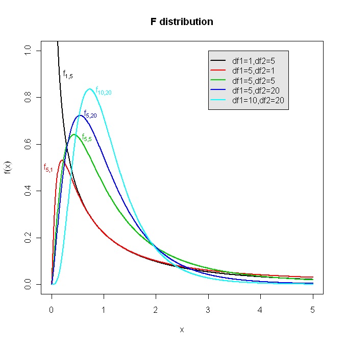
The distribution of the ratios of sample variances and this assumes the shape of the F distribution. The F distribution however does not have a single shape for any given mean and standard deviation, as does the normal curve, nor does it have a symmetrical shape that grows 'taller' as sample size increases, as is the case with the t-distribution. The F-distribution is affected by the size of both samples being tested and takes on a variety of shapes according to the number of degrees of freedom associated with each sample variance.
F curves are not symmetrical. They are usually demoted as Fx,y where x is the number of degrees of freedom for sample 1 and y is the number of degrees of freedom of sample 2 (degrees of freedom are derived from sample size)
F curve F1,5 is a downwards sloping curve while F5,1 is a skewed bell-shape curve. In short, the two curves are not reversible. See diagram: F distribution.
The tables of areas under the F-curve are laid out in accordance with
this non-reversible property of the F distribution and in order to find the correct critical value it is imperative to denote the sample with the largest variance as sample 1. (Note: the sample with the largest variance will not necessarily be the sample with the largest size.)
The F distribution is the distribution of the ratio of population variances, thus:
F=population variance1/population variance2
= σ12/σ22
An unbiased estimate of var1 and var2 can be derived from the sample variances with the sample variance adjusted by a factor of n/(n-1)
Thus
F= sample var1(n1/(n1-1))/sample var2(n2/(n2-1))
Assumptions
The F-test is applicable only when the populations from which the two sample variances are taken are both normally distributed: unless the parent populations are both normal the F distribution does not hold for the ratio variance1/variance2.
Testing statistic
The F testing statistic (denoted with degrees of freedom x for largest variance, y for smallest)
Fx,y = (sample var1(n1/(n1-1)))/(sample var2(n2/(n2-1)))
where:
sample var1 is the largest sample variance
sample var2 is the smallest sample variance
n1 is the size of the sample with the largest variance
n2 is the size of the sample with the smallest varianee
x, is the number of degrees of freedom associated with sample one
y is the number of degrees of freedom associated with sample two.
See NOTE on degrees of freedom
Critical values
When undertaking an F test it is most usual to carry out a one-tail test, i.e. to see whether one variance is significantly larger than the other. However it is possible to carry out a two-tail test and the derivation of the critical values for both cases is explained below.
(a) One tail test.
Establish which sample has the larger variance, call it sample 1. The number of degrees of freedom associated with sample 1 will be equal to the size of sample 1 minus 1 (thus x degrees of freedom = n1-1). Similarly, for degrees of freedom of sample 2 (y = n2-1).
Having decided on the significance level, use a table of F critical values and read off the critical value by locating the x degrees of freedom value in the top row of the table and the y value in the first column and finding where they intersect in the body of the table. (A computer program will generate both the appropriate degrees of freedom and the critical value)
Once this critical value has been located the decision rule for a one-tail test is that the null hypothesis (H0) is rejected if the calculated value of F is greater than the critical value of F.
(b) Two-tail test.
The upper critical value is located in the same way as for a one-tail test (above) above. However, a two-tail test also need a lower limiting value. Because of the shape of the F distribuition the lower value is not just a negative of the upper version (as it would be in a z or t test). The lower limiting value is found by looking up the "reverse value" of F and then taking the reciprocal of it. The lower limiting value is therefore equal to:
1/Fx,y
One per cent and five per cent significance tables are usual for F distributions but are of a one-tail type (i.e. when looking up a critical value the 1% is located solely in one tail). Thus when they are used for two tail tests they are in fact doubling the level of significance.
H0 is rejected if the calculated value of F exceeds the upper limit or is less than the lower limit.
A two-tail test compares the ratio of variances in two directions. First, to see if it is 'significantly large' and, second, to see if it is 'significantly small'. A significantly small F value indicates that the two variances are too close, i.e. unlikely given the sample sizes (indicating that the two samples are unlikely to have been drawn randomly).
Worked example (conventional one-tail F test)
A teacher at a comprehensive school teaches mathematics to two different classes. Both classes are mixed ability. The teacher divides the combined set of pupils into two groups, A and B, at random. The teacher enters group A for an examination with one Board and group B with a different Board. The average marks for both groups are fairly close, but the standard deviation of the 36 students in group A was only 5% whilst the standard deviation of the 31 students in group B was 12% . Is there a significant difference in the variability of the marks on the two Boards.
Hypotheses:
H0:σ12=σ22 or var1 = var2
HA:H0:σ12>σ22 or var1>var2
One-tail test to see if the student marks for Group B are significantly larger variance than for Group A.
Significance level: 5%
Testing statistic: Fx,y = sample var1(n1/(n1-1))/sample var2(n2/(n2-1))
Critical value: x=31-1=30 y=36-1=35
Therefore critical Fx,y = critical F30,35
Decision rule: reject H0 if F30,35>1.79 (derived from tables of F values as most popular value)
The critical value is actually disputed. The folowing sources provided different critical values for F30,35.
University of Baltimore =1.79 (accessed 30 April 2020)
University of Texas at Austin, Department of Mathematics = 1.76 (accessed 30 April 2020)
Computation:
F30,35 = (sample var1(n1/(n1-1))/sample var2(n2/(n2-1)))
s1 = 12, thus var1 =144
s2 = 5, thus var2 =25
n1 = 31
n2 = 36
F30,35 = (144(31/30))/(25(36/35)) = 148.8/25.71 = 5.79
Decision: Reject the null hypotheses (H0:σ1=σ2) 5.79 > 1.79 (the critical value of F in a one-tail test at 5% significance level); the two Boards have have significantly different population variances: student mark variability is much greater for the Board taken by group B than the Board taken by group A.
Worked example (less usual two-tail F test)
The returns of two area managers working for a large company were investigated. Each manager supervised 31 selling agents. The total sales of eaeh area for the first quarter of the year were shown to be almost identical. The firm was concerned that there had been some collusion between the area managers to reduce inter-area competition. As a check the variation in sales per agent in each area was investigated. Area A had an agent sales variance of £100 while area B had a variance of £110. Is there any reason to consider that the difference in the variances is significant?
This example is concerned with the ratio of the variances in both directions. First, to see if it is 'significantly small' and, therefore, indicative of confirmation of the firm's belief about collusion, Second, to see if the ratio of variances is 'significantly large' thereby rejecting the firm's fears.
Hypotheses:
H0:σ12=σ22
HA:H0:σ12≠σ22
Two-tail test to see if the variances differ significantly.
Significance level: 5% (but actually doubled as 5% for each tail due to limitations of available tables), thus 10%
Testing statistic: Fx,y = sample var1(n1/(n1-1))/sample var2(n2/(n2-1))
Critical value: x=31-1=30 y=31-1=30
Therefore critical Fx,y = critical F30,30 (upper limit) = 1.84 and critical Fy,x is F30,30 (lower limit) = 1/1.84 = 0.54
Decision rule: reject H0 if F30,30>1.84 or F30,30>0.54
The critical value for 2% (i.e 1% in each tail, also available from tables, would be 2.39)
Computation:
F30,35 =( sample var1(n1/(n1-1))/sample var2(n2/(n2-1)))
var1 =110
var2 =100
n1 = 31
n2 = 31
F30,30 = 110(31/30)/100(31/30) = 100/110 = 1.1
Decision: The null hypotheses (H0:σ12=σ22) cannot be rejected at a 90% level of confidence as 0.54<1.11<1.84 (the critical value of F in a one-tail test at 5% significance level). Thus neither team has a significantly more variable sales record; nor is the ratio of the variances signicantly small, so collusion is not attested to by the analysis.
Unworked Examples
1. Two groups of 26 students were given an identical statistics test scored out of 100. Group One had a variance of 49. Group Two had a variance of 30. Does the variance of the two groups vary significantly?
2. Two road haulage companies, both with the same type of lorry, were investigated to see how much their loads varied. A sample of 101 journeys taken at random showed that company A's lorries carried an average load of 12.94 tons, with a standard deviation of 3 tons. A sample of 51 journeys for company B had an average of 10.09 tons and a standard deviation of 2.12 tons. Is the variability of loads carried by road haulage company A significantly different from the variability of loads carried by company B?
|